Dense Photometric Stereo
Introduction
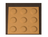
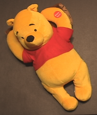
This project is the implementation of this paper: Dense Photometric Stereo Using a Mirror Sphere and Graph Cut. Basically it uses a dataset with many photos of the same object taken under different light directions (photos and corresponding light directions are given) to reconstruct a 3D model of the object. Steps strictly follows the paper, here I only briefly describe the steps, please refer to the paper for more details. Implementation is done on Matlab, and code can be downloaded here, and corresponding libraries used are stated in the README.
Step 1: Uniform resampling
Start with an sub-divided (4 times) icosahedron, finding the nearest icosahedron vertex L_o compared with each light direction L_i. Then interpolate the image I_o at L_o by:
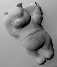
Step 2: Find denominator image
Denominator image will be used for finding normals in the next step. Ideally, the denominator image should cancel out the surface albedo by producing ratio images, and it should be least affected by shadows and highlights.
The selection step is: for each pixel (i,j), we sort the intensity of corresponding pixels over all images to have a full rank at each location. Then count the total number of pixels in each image that satisfies pixel_rank > 70th percentiles. Calculate the mean rank of these pixels for each images, and only keep those images that mean rank < 90th percentiles. Then choose the image with maximum number of pixels satisfying rank condition to be the denominator image.
Step 3: Initial normal estimation
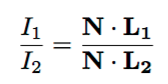
The objects are supposed to be nearly Lambertian. To cancel out surface albedo, divide each image by the denominator image to get k-1 ratio images (suppose in total k images). Each equation is:
Step 4: Refining normal by MRF graph cut
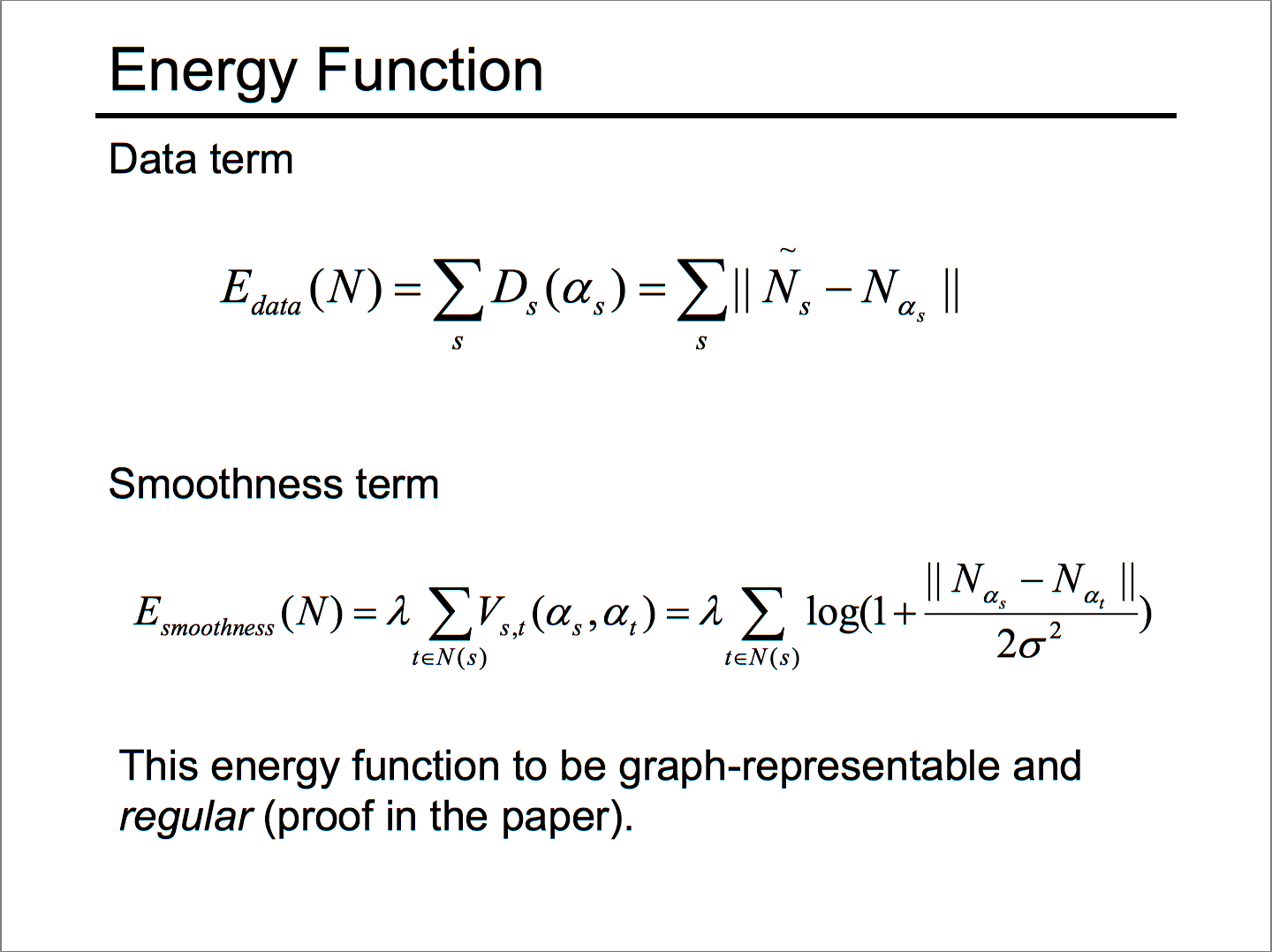
Technical details please see the paper. For implementation, basically input initially estimated normal and set MRF energy for graph cut problem as:
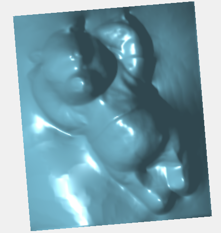
Step 5: Reconstruct 3D models
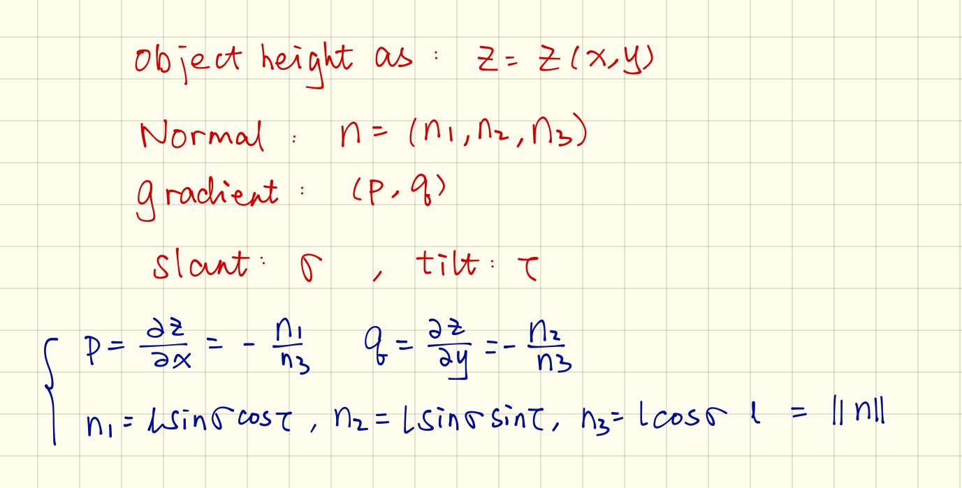
Given the refined normal on each pixel, I transferred it to gradient by the following:
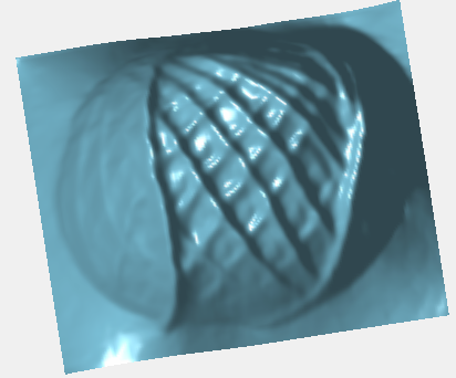
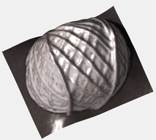
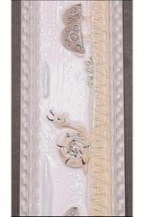
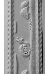
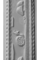
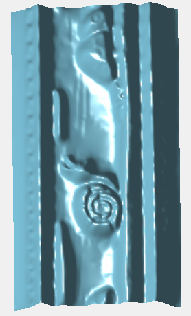
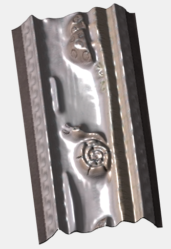
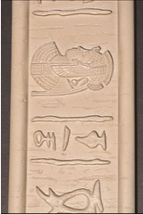
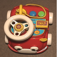
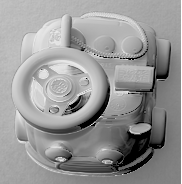
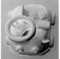
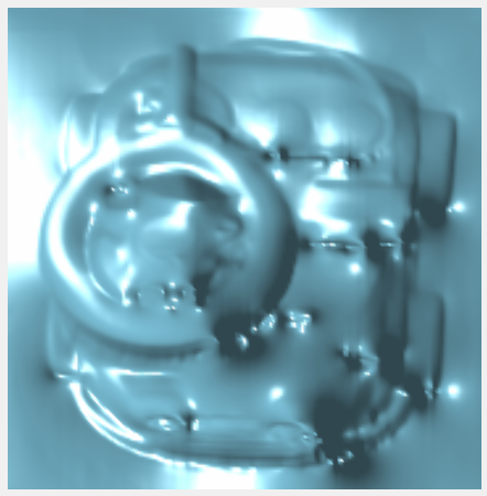
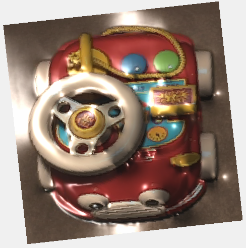
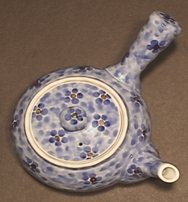
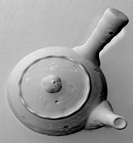
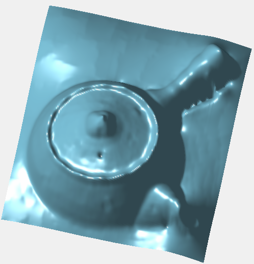
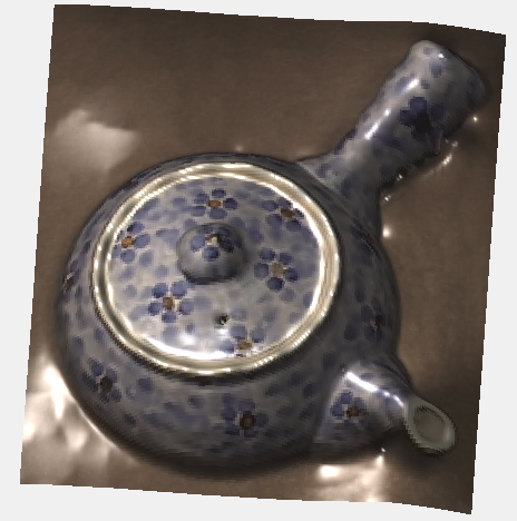
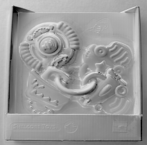
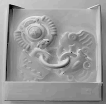
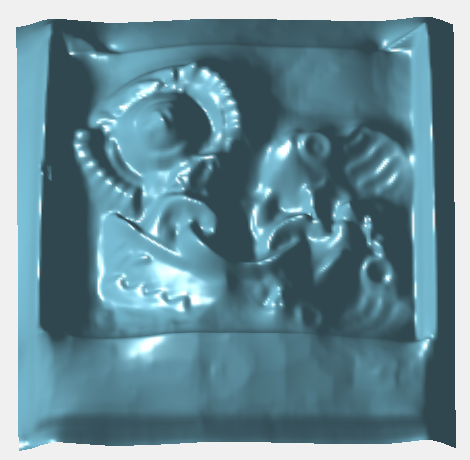
Results
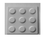
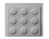
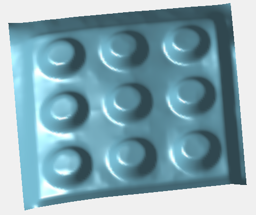
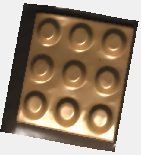
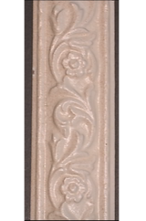
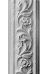
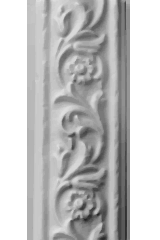
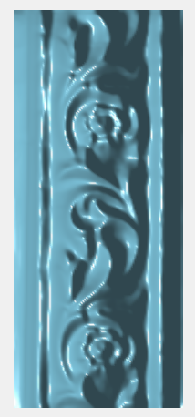
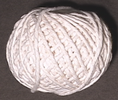
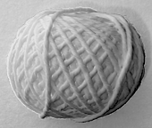
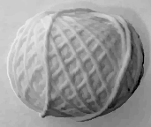
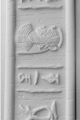
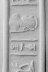
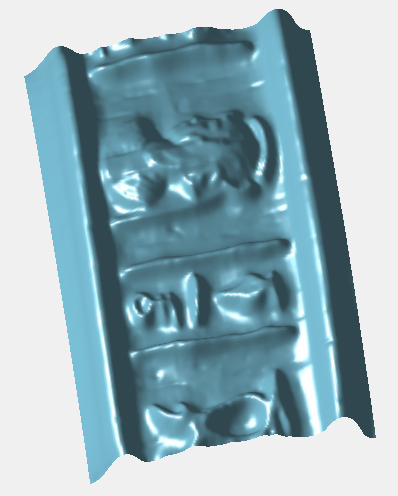
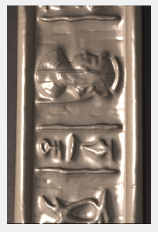
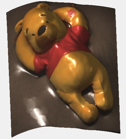
From left to right:
denominator image selected, initial normal, refined normal, 3D model, textured 3D model
 |
 |
 |
 |
 |
 |
 |
 |
 |
 |
 |
 |
 |
 |
 |
 |
 |
 |
 |
 |
 |
 |
 |
 |
 |
 |
 |
 |
 |
 |
 |
 |
 |
 |
 |
 |
 |
 |
 |
 |
 |
 |
 |
 |
 |
Reference
- Paper: Dense Photometric Stereo Using a Mirror Sphere and Graph Cut
- CK Tang's COMP5421 Notes at HKUST
- How to use GCO library (good resource, but in Chinese)
- Something about graph cut and GCO library